This part of our site will deal with image processing. After a short introduction to common methods, we will present the program Qlisp. You will find concrete examples at the end of this chapter.
In image analysis, we distinguish two different theories: Mathematical morphology and signal processing.
The principal transformations of mathematical morphology are intersections, unions and translations of sets. By their combination, you can obtain complex functions. For example, an alternate sequential filter of the size 11x11 carries out 240 translations, 120 intersections and 120 unions. The morphological transformations have well defined mathematical properties and their application gives stable and predictable results.
Many efforts have been made to shorten the computing time of some complex functions. The "watershed" or the "numerical reconstruction" requires now only a few milliseconds by using queue-based algorithms.
The theory of signal processing describes mathematically the behaviour of linear and time-invariant systems. This theory is well researched and applied in very different fields: Electrical engineering, biology, medicine and seismology, to mention only some. In the Fifties, digital treatment of signals was introduced. The power of the latest generation of microcomputers makes it possible today to treat images in reasonable computing time.
The principal transformations are the convolution and the Fourier transformation. The comprehension of these tools is less intuitive and requires good theoretical knowledge.
We think that an advantage for industrial control is the non-linearity of morphological functions. Starting from the original image, you eliminate - with each transformation - useless information by keeping the features that you want to extract.
In other fields, however, like the visual improvement of images, the description of contours or compression, the methods of signal processing are incontestably better adapted.
The examples at the end of this section will show you typical applications for mathematical morphology and for signal processing. But initially, we would like to present you the tool that we use for image processing.
The first version of Qlisp was programmed in 1991 on the image processing station Q570 of Cambridge Instruments: We combined the library of the Q570 with the Lisp interpreter. The PhD thesis "Morphologie Mathématique Appliquée au Contrôle Industriel de Pièces Coulées, T. Jochems, School of Mines, Paris" describes the design and the use of this version.
The fast growth of computers' power was the basis of a second version. The transformations carried out electronically on the Q570 were replaced by functions coded in C. Programmed on an Alpha station of DEC, Qlisp is used from now on for teaching artificial vision at the Engineering School IMERIR, Perpignan.
Since then, the system has been widening continuously and has the following features today:
For industrial applications, the routines of image analysis are often used in a specific data-processing environment, which ensures the stability and the coherence of these applications. For this reason, we decided to split up Qlisp in two distinct parts:
a library of image analysis routines programmed in C. This library is completely independent of Lisp; it has already been used with various programming tools and operating systems (C++Builder, Bc5, GCC, Linux, Unix on DEC);
a thin layer which connects Lisp to this library.
The advantage of this approach is that you can initially develop and test applications with the Lisp interpreter. This decreases appreciably the length of this period. As a second step, you can export the resulting prototype to your industrial application.
Here is the list of C routines that you dispose of after having downloaded Qlisp.
|
Fichier |
Fonctions |
|
intern.cpp |
extern
void imainit(); |
|
base.cpp |
extern
int binrpix(int id,int x,int y); |
|
trans.cpp |
extern
void bingrey(int bin,int gout); |
|
queue.cpp |
extern
void qinit(); |
|
measure.cpp |
extern
void greymeas(int id,int *min,int *max,double *mean); |
|
signal.cpp |
extern
void convh(int gin,int gout,...); |
|
io.cpp |
extern
void loadcamera(char *name); |
|
color.cpp |
extern
void colgrey(int col, int red, int green, int blue); |
We use Qlisp for teaching image analysis. Its hierarchical structure, explained in the next figure, is the main reason for its good suitability for education.
In the lowest layer, the functions are coded in C because of the speed of this language. There is no pedagogical interest for beginners in image analysis to realize these functions, the time required being too long.
In the Lisp layer, the basic functions can be combined to obtain new, more complex and more powerful methods. This property of Qlisp is well adapted to mathematical morphology: An erosion of size n, for example, is calculated by applying n times an erosion of size 1 (decomposition of the structuring element); an opening is defined as an erosion followed by a dilation with the transposed structuring element. The following table shows the coding of three new transformations. The functional character of Lisp simplifies programming.
|
Function |
Coding in Lisp |
|
geodesic dilation |
(defun gdsdilation(ima mask se size) |
|
morphological opening |
(defun opening(ima se size) |
|
gradient |
(defun gradient(ima &key (se se-c) (size 1)) |
The participants of the courses work on the Lisp layer and in this way put the theory into practice. In the current system, more than 100 transformations are defined in Lisp.
In the application layer, you can finally solve real and complex problems while using the basic library and the transformations coded in Lisp. In the following chapter, we will show three examples, which are also treated in our courses.
In this chapter, we will illustrate the various approaches of image analysis with some examples. All results are calculated with the Qlisp system.
This example shows line detection on a metal sheet. It was studied at the ENSMP by A. Tuzikov for the Belgian company OCAS.
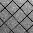
Image (1) shows a metal sheet (25x25 mm) on which black lines have been traced. The interest is the automatic detection of these lines after deforming the sheet by pressure. The data thus obtained is used to optimize the tool of deformation.
|
|
|
|
|
|
1) original |
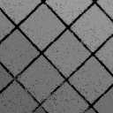
2) opening |
3) threshold |
|
|
|
|
||
|
4) binary filter |
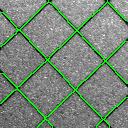
5) result |
||
The treatment starts with a noise filter (2). A "top hat" eliminates then the effect of heterogeneous lighting. A consecutive threshold produces image (3). A binary filtering of noise (4) and a "skeleton by influence zone" finish the treatment. The result is shown in image (5).
This example shows well the philosophy of morphological filtering: You remove more and more information (noise, gray-levels, size) by keeping only the desired features.
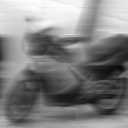
This example shows an application of signal processing. Image (1) presents the original image captured by a camera, which has a defect in the video amplifier. Although we simulated this defect, it could be a real problem, see Apollo or Hubble...
|
|
|
|
1) original |
2) characteristics |
|
|
|
|
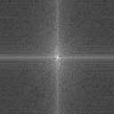
3) spectrum |
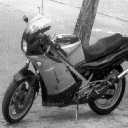
4) result |
We need a description of the defect. In our case, we acquire the image (2) with only one lit-up central point. This image thus represents the impulse response of the defective camera. We calculate then the spectrum (3) of image (1) and the spectrum of the impulse response. We finish by dividing these spectra and applying the inverse Fourier transformation. The result (4) is not fuzzy any more. Signal processing needs a lot of computing time: 85ms for this example.
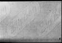
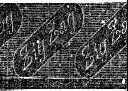
This example shows the recognition of filigrees. It was resolved in a school project by a group of 4 students at the Engineering School IMERIR.
|
|
|
|
1) original |
2) amplified contrast |
|
|
|
|
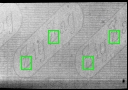
3) sample |
4) result |
Image (1) shows the filigrees acquired by a black-and-white camera. The first step consists in improving and stabilizing the contrast of this image. We use a "top hat" and "histogram imposing " and get the result (2). Here we will seek a sample (3), which shows a characteristic part of the filigree. This image was stored before in a database. The result (4) illustrates that the sample is detected 4 times in the original image. The recognition of the sample is carried out by an accelerated correlation between the images (2) and (3), the processing time is 25ms for the complete process.
Perhaps you would like to test yourself the image analysis transformations. You could download Qlisp and test at home the examples contained in this program. And you could try to treat your own images.